Questions
Multiple fill-in-the-blank
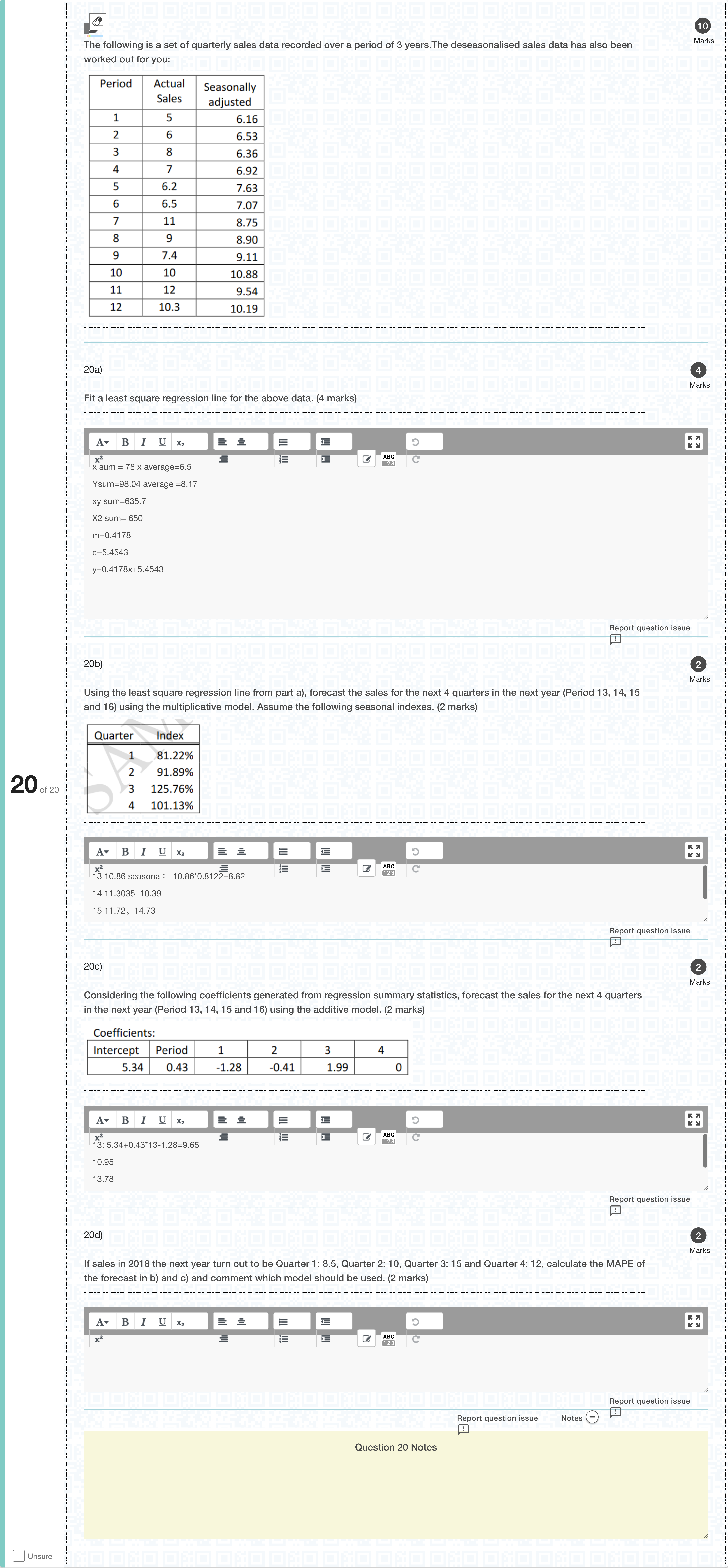
The following is a set of quarterly sales data recorded over a period of 3 years.The deseasonalised sales data has also been worked out for you:[Fill in the blank] Fit a least square regression line for the above data. (4 marks)[Fill in the blank] Using the least square regression line from part a), forecast the sales for the next 4 quarters in the next year (Period 13, 14, 15 and 16) using the multiplicative model. Assume the following seasonal indexes. (2 marks)[Fill in the blank] Considering the following coefficients generated from regression summary statistics, forecast the sales for the next 4 quarters in the next year (Period 13, 14, 15 and 16) using the additive model. (2 marks)[Fill in the blank] If sales in 2018 the next year turn out to be Quarter 1: 8.5, Quarter 2: 10, Quarter 3: 15 and Quarter 4: 12, calculate the MAPE of the forecast in b) and c) and comment which model should be used. (2 marks)[Fill in the blank]

View Explanation
Verified Answer
Please login to view
Step-by-Step Analysis
The question presents a multi-blank forecasting problem with four parts. We will consider each blank sequentially and explain the reasoning behind the provided answers, while noting how each result is obtained and where common pitfalls might lie.
Part a — Fit a least squares regression line for the above data
- The task is to fit a simple linear regression to the deseasonalised quarterly sales data, treating time (e.g., period number) as the predictor and the deseasonalised sales as the response.
- The provided answer is: y = 0.4178x + 5.4541 (or 5.4543 in another variant). This form specifies a slope (approximately 0.418) and an intercept (approximately 5.454).
- Why this is reasonable: In a regression framework, the slope represents the average change in the deseasonalised sales per one-quarter step, while the intercept shifts the line to the appropriate scale. A positive slope around 0.42 indicates a modest increasing trend over time, which is plausible for many seasonal demand series that gradually rise.
- How you would verify: compute the regression using the period index (1,2,3,…) as the predictor and the deseasonalised values as the response, and check that the estimated coefficients minimize......Login to view full explanationLog in for full answers
We've collected over 50,000 authentic exam questions and detailed explanations from around the globe. Log in now and get instant access to the answers!
Similar Questions
Which of the following forecasting methods requires the least amount of past data to produce a forecast for the next period?
Consider the following questions relating to time series.Answer the following questions, and show all working at all stages in every question.Give answers to at least 3 significant figures and at least 2 decimal places.[Fill in the blank] Consider the following time series data of y as a function of (time) t.t y2015 1002016 1102017 1052018 1112019 116Setting alpha = 1/2 = 0.5, give the exponential smoothing forecasts for 2016, 2017 and 2018.Then give the mean absolute percentage error (MAPE) for these 3 forecasts.[Fill in the blank] Consider some data of values X and Y, where we plan to perform a linear regression and say that Y is a function of X. X can also be regarded as equivalent to time, t.Let's suppose that we have N = 10 values of (X, Y). We will not provide these 10 values. Instead, we provide the following. We give the sum of the values of X, and the sum of the values of Y, and the sum of the values of (XY), the sum of the values of (X2), and the sum of the values of (Y2). We will then ask you to give the gradient and the Y-intercept for the linear regression.Sum(X) = 55Sum(Y) = 110Sum(XY) = 762Sum(X2) = 385Sum(Y2) = 1540What is the gradient for the linear regression?What is the Y-intercept for the linear regression?[Fill in the blank]
Table 8.9 The manager of a pizza shop must forecast weekly demand for special pizzas so that he can order pizza shells weekly. Recent demand has been: WEEK No. Special Pizzas 1 30 2 45 3 33 4 36 5 35 6 40 Use the information from Table 8.9. The pizza shop manager believes that a combination forecast might improve her ability to predict future demand, and thus improve keeping fresh ingredients on hand. She decides to use the 3-week weighted moving average and exponentially smoothed average forecast, giving them equal weight. The 3-week weighted moving averages are .6 for the most recent period, .25 for the second most recent period, and .15 for the third most recent period. The smoothing constant is .10 and the previously forecasted demand for week 6 was 39.28 pizzas. What is her forecast for week #7?
With the multiplicative seasonal method of forecasting:
More Practical Tools for Students Powered by AI Study Helper
Making Your Study Simpler
Join us and instantly unlock extensive past papers & exclusive solutions to get a head start on your studies!