Questions
Single choice
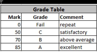
To return (display) excellent from the VLookup table shown, the col_index_num in the IF function arguments should be
Options
A.a. 1
B.b. 2
C.c. 3
D.d. 4
View Explanation
Verified Answer
Please login to view
Step-by-Step Analysis
To interpret this VLOOKUP scenario, first recall how VLOOKUP works: you search for a value in the first column of a table and return a value from a specified column in the same row, using the col_index_num to pick the target column.
Option a: 1. This would return the value ......Login to view full explanationLog in for full answers
We've collected over 50,000 authentic exam questions and detailed explanations from around the globe. Log in now and get instant access to the answers!
Similar Questions
P Q R 2 Target ISO Code Better than the Target 3 85 BEL FALSE Ruijing wants to check whether the country whose ISO code is entered in Q3 has better air quality than the target in P3. She entered a formula in R3. R3 should return logical: TRUE if the country's AIR value (i.e., its air quality index reported in the appropriate cell in column M) is greater than the target in P3. FALSE otherwise. Note: The screenshot shows Q3 is BEL (i.e., Belgium). But, Q3 can be any ISO code; R3 should always evaluate based on the code in Q3 and the target in P3. Complete the formula in R3 by filling the blanks below. =XXX(XXX,B2:M181,12,XXX)XXXP3 (no $ signs and no blank spaces in your formula) In each blank, you may use only one of the following: a function name, a cell reference, a value (logical, text, or number), or a logical comparison operator. =[Fill in the blank] ([Fill in the blank] ,B2:M181,12,[Fill in the blank] )[Fill in the blank] P3
T/F To answer the above question, one can also use the following formula. =VLOOKUP(A26,A2:C23,2,FALSE)&" "&"won the cup in"&" "&A26&"." Note: The " " instances represent strings consisting of a single blank space.
Alex wants to calculate the income tax payable in British Columbia (federal + provincial combined) using the table below. Alex enters the taxable income in cell B15 and needs to calculate the tax payable in cell B16 using a VLOOKUP-based formula. The formula combines: Example: If Alex’s income is $100,000, it falls in the bracket starting at $98,560 with a 32.79% marginal rate. Tax = ( Income − Bracket start ) × Marginal rate percentage + Base tax ($24,712) = (100,000 − 98,560) × 32.79% + $24,712 = $25,184.176 In cell B16, Alex enters the following formula: =VLOOKUP(B15,A3:C12,___) * (B15-VLOOKUP(B15,A3:C12,___)) / ___ + VLOOKUP(B15,A3:C12,___) Please fill the blanks to complete Alex's formula. =VLOOKUP(B15,A3:C12,[Fill in the blank], ) * (B15-VLOOKUP(B15,A3:C12,[Fill in the blank], )) / [Fill in the blank], + VLOOKUP(B15,A3:C12,[Fill in the blank], )
In an attempt to impress his goggles-wearing doctor supervisor, Ryan created an inventory look-up tool on the Excel datasheet, called GoggleDoc (which stands for Goggles Doctor, not to be confused with GoogleDoc!). If one types the item number into cell B2, the tool will automatically return the area of the item in cell B4, and whether it is a sterile environment in cell B5. Select the correct pair(s) of formulas for cells B4 and B5. There is AT LEAST ONE correct option, but you MUST SELECT ALL correct options. [Note that the number of marks allocated to this question does NOT necessarily correspond to the correct number of options.]
More Practical Tools for Students Powered by AI Study Helper
Making Your Study Simpler
Join us and instantly unlock extensive past papers & exclusive solutions to get a head start on your studies!