Questions
COMM_V 205 101 102 103 2025W1 In-class Exercise (ICE) 5
Multiple choice
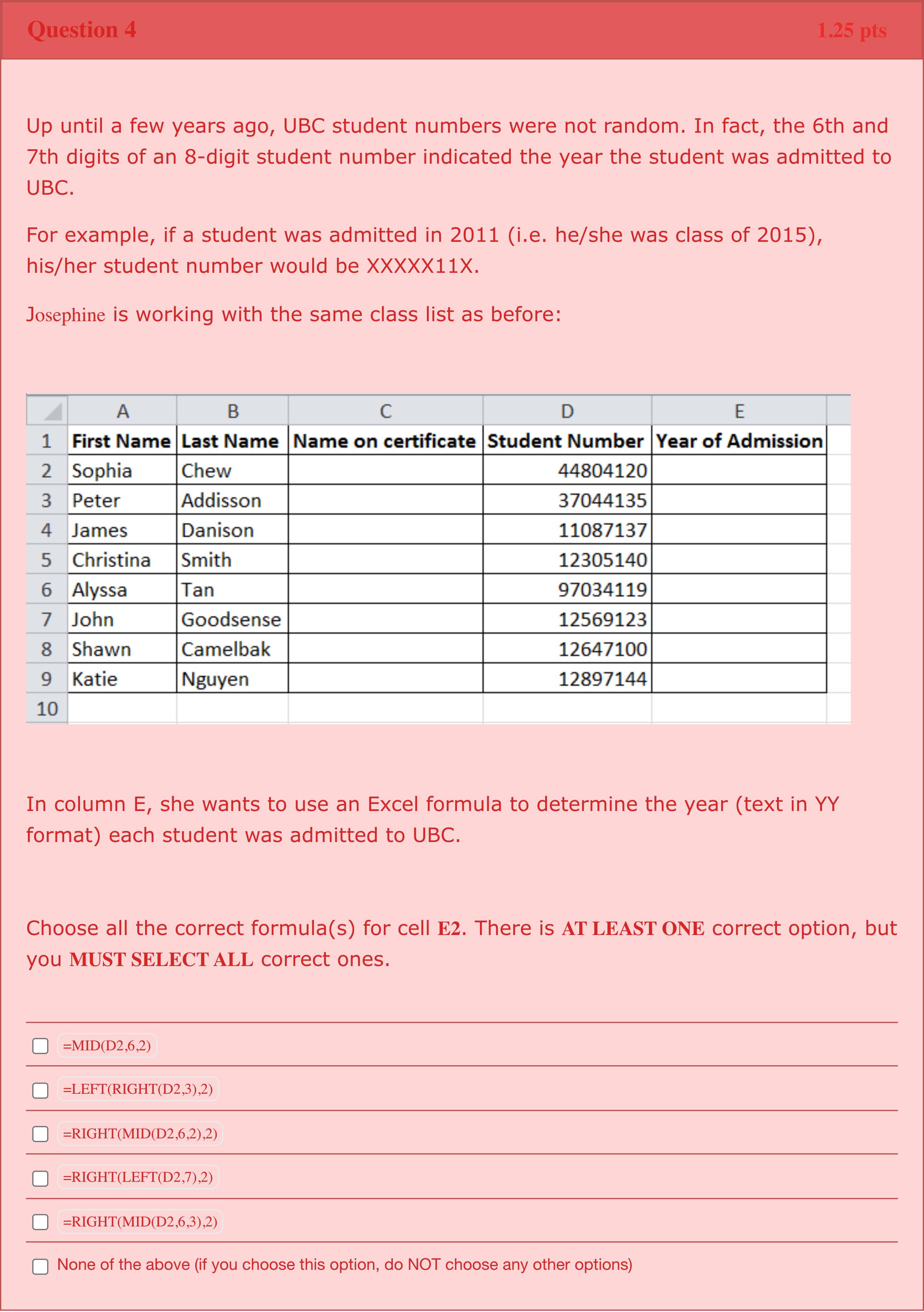
Up until a few years ago, UBC student numbers were not random. In fact, the 6th and 7th digits of an 8-digit student number indicated the year the student was admitted to UBC. For example, if a student was admitted in 2011 (i.e. he/she was class of 2015), his/her student number would be XXXXX11X. Josephine is working with the same class list as before: In column E, she wants to use an Excel formula to determine the year (text in YY format) each student was admitted to UBC. Choose all the correct formula(s) for cell E2. There is AT LEAST ONE correct option, but you MUST SELECT ALL correct ones.
Options
A.=MID(D2,6,2)
B.=LEFT(RIGHT(D2,3),2)
C.=RIGHT(MID(D2,6,2),2)
D.=RIGHT(LEFT(D2,7),2)
E.=RIGHT(MID(D2,6,3),2)
F.None of the above (if you choose this option, do NOT choose any other options)
View Explanation
Verified Answer
Please login to view
Step-by-Step Analysis
The task is to extract the two-digit year (YY) encoded in positions 6 and 7 of an 8-digit student number stored in D2.
Option 1: =MID(D2,6,2) — This directly grabs 2 characters starting at position 6, which are exactly the 6th and 7th digits. This is correct.
Option 2: =LEFT(RIGHT(D2,3),2) — Right(D2,3) takes the last 3 dig......Login to view full explanationLog in for full answers
We've collected over 50,000 authentic exam questions and detailed explanations from around the globe. Log in now and get instant access to the answers!
Similar Questions
True/False: The two formulas =LEFT(RIGHT(A2,5),5) =MID(LEFT(A2,5),1,5) will result in the same answer for any value of cell A2.
You typed TRUE and executed in A1. Then, you typed LOVE and executed in B1. A B 1 TRUE LOVE 2 XXXXXXXXXXX Then, you typed and executed the following formula in A2. =TRIM(CONCATENATE(TRIM(A1)," ",B1)) where " " is a text with only single blank space. What is the output returned in A2.
Consider a fictional (and artificial) language called Galitéis. Galitéis and English share many similarities. Every English word that contains "ble" (at the beginning, in the middle, or at the end) will translate to "vel." For example, the English word "doable" will translate to "doavel" in Galitéis. Two other examples: the English word "bleed" will translate to "veled" in Galitéis; the English word "trebled" will translate to "treveld" in Galitéis. You are given the following table and are asked to translate each English word to Galitéis (that is, to complete column B, cells B2:B7). You will type up your formula in cell B2, and then drag the formula down to cell B7. The formula with some redaction looks like this: =XXX(A2, XXX("XXX",A2),3,"XXX") Complete the following formula for cell B2: Note: Unless absolutely necessary, do NOT leave any spaces in your formula. Do NOT use any additional brackets ( ) in your formula either. =[Fill in the blank], (A2,[Fill in the blank], ("[Fill in the blank], ",A2),3,"[Fill in the blank], ")
You first wrote the following formula in T2 to indicate if the first game (whose name is in R2) was released earlier than the second game (whose name is in S2): =IF(VLOOKUP(R2,B2:G1301,6,FALSE)<VLOOKUP(S2,B2:G1301,6,FALSE),"YES","NO") When you were testing the formula, you entered the two game names as follows: Given that Oct 25, 2005 (the released date of Grand Theft Auto: Liberty City Stories) happened before Sep 27, 2016 (the released date of FIFA 17), the T2 should have indicated “YES”, not “NO” as you see above. While you were thinking about it, you realized that the format is MM/DD/YYYY in G column. Therefore, although Oct 25, 2005 (the released date of Grand Theft Auto: Liberty City Stories) is earlier than Sep 27, 2016 (the released date of FIFA 17), ="10/25/2005"<"09/27/2016" would result in FALSE. Therefore, you cannot use the date format used in G column. You decided to create a new variable called r_date (stored in the L column) by reorganizing characters in the values in column G. You will write a formula in L2 and drag it down to L1301. The formula in L2 that you are asked to complete below will refer to G2 and will produce reorganized released date (i.e., r_data for the game in row 2) that has only 8 characters, each of which can only be 0, 1, 2, 3, 4, 5, 6, 7, 8, or 9. That is, you need to reorganize the existing characters except “/” to create 8-character-long r_date value. =XXX(XXX(G2,XXX),XXX(G2,XXX)&XXX(G2,XXX,XXX)) =[Fill in the blank], ([Fill in the blank], (G2,[Fill in the blank], ),[Fill in the blank], (G2,[Fill in the blank], )&[Fill in the blank], (G2,[Fill in the blank], ,[Fill in the blank], )) With the new column L (remember after typing in L2, you have copied all the way through L1301), if you have also revised the formula in T2 to refer to G column instead of L column as follows: =IF(VLOOKUP(R2,B2:L1301,11,FALSE)<VLOOKUP(S2,B2:L1301,11,FALSE),"YES","NO") You will get the right result for the two games tested previously as shown below: In each blank, you can either use a function name or number.
More Practical Tools for Students Powered by AI Study Helper
Making Your Study Simpler
Join us and instantly unlock extensive past papers & exclusive solutions to get a head start on your studies!