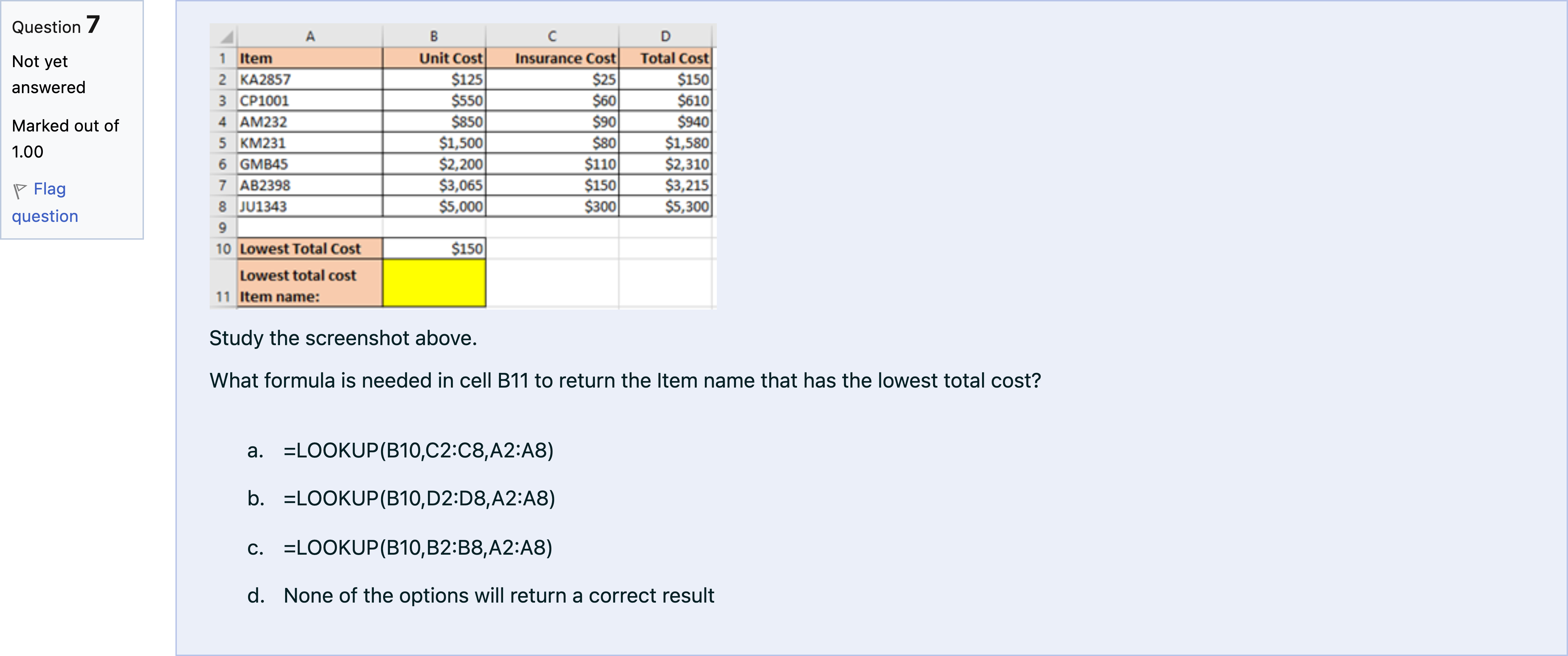
Study the screenshot above.What formula is needed in cell B11 to return the Item name that has the lowest total cost?

Question

BlackTom AI · Accepted Answer

Let's analyze each option by checking how the LOOKUP function works in this context.
Option a: =LOOKUP(B10,C2:C8,A2:A8)
- Here, the lookup_vector is C2:C8, which contains Unit Cost values, not the column that holds the total cost. Since we want to match the item by its total cost, using C2:C8 as the lookup_vector will not align with the intended lookup. This will yield an incorrect mapping between the found total cost and the item name. 
Option b: =LOOKUP(B10,D2:D8,A2:A8)
- This uses D2:D8 as the lookup_vector, which corresponds to the Total Cost column, and A2:A8 as the result_vector, which holds the Item names. Given that B10 contains the lowest total cost, this arrangement correctly finds the item name whose total cost matches the lowest value. This is the appropriate structure for returning the item name associated with the minimum total cost.
Option c: =LOOKUP(B10,B2:B8,A2:A8)
- In this case, the lookup_vector is B2:B8 (Unit Cost), while B10 is the lookup_value. This mismatches the data layout, because B10 is a total cost value, not a unit cost. The function would attempt to find a unit cost that equals the lowest total cost, which is incorrect and will yield erroneous results for the item name.
Option d: None of the options will return a correct result
- Since option b correctly maps the lowest total cost to its corresponding item name, this statement is not true. The correct approach is demonstrated in option b.
In summary, option b uses the proper pairings for lookup_vector and result_vector to return the item name associated with the lowest total cost, whereas options a and c misalign the columns, and option d contradicts the valid approach provided by option b.

FNDN Computing for Business 2025 STD O1

Study the screenshot above.What formula is needed in cell B11 to return the Item name that has the lowest total cost?

查看解析

登录即可查看完整答案

类似问题

A B C D E F 1 Score 0% 60% 70% 80% 90% 2 Letter E D C B A Given the table above, which formula will give the letter grade if the score is located in cell H6, and the score is not an exact match?

A B C D E F 1 Score 0% 65% 75% 85% 95% 2 Letter F D C B A Given the table above, which formula will return the letter grade if the score is in cell G4 and may not exactly match one of the percentage breakpoints?

Study the screenshot above.What formula is needed in cell B11 to return the Student name that has the lowest English mark?

Look up the Employment Status from the Exit Poll Respondents worksheet. How many of the respondents on the "Conversion" worksheet are Retired?

For the HLOOKUP function, the lookup_value must be in the first row of the table array.

Complete the following statement: The lookup vector in a LOOKUP function:

Study the screenshot above.What formula will need to be entered in cell B11 to return the Student name that has the highest Computing mark?

更多留学生实用工具

考试浏览器助手

风格化写作助手

论文查重助手

文献引用助手

课堂转译助手

课堂笔记助手

Quiz搜索助手

学校历年真题

智能刷题助手

智能匹配练习

希望你的学习变得更简单